Learn about techniques for producing a high vacuum.
Learn about techniques for measuring pressure.
Perform the thermal evaporation of thin metal (aluminum) films.
Study the operation of quartz crystal thickness monitors.
Learn how to use a lock-in amplifier to detect small signals.
Study the relationship between measured resistances to parameters of thin film structure.

Introduction to Thin Film Deposition

A thin film is a film of material only a few microns or nanometers thick, deposited on a substrate, such as in the technology for making integrated circuits. Thin film deposition of various materials plays a crucial role in the fabrication of modern microelectronic devices and enables investigations of fundamental physical principles. In this experiment, we used a technique called thermal evaporation to controllably deposit thin films of aluminum onto glass with thicknesses of 300 angstroms and 600 angstroms. The thin films were deposited with a shadow mask configured for subsequent electrical measurements of the resistance of the thin films. We used these measurements to determine the Resistivity of aluminum and compared it to the accepted value.

Thermal Evaporation Method

Thermal Evaporation Method is one of the many techniques used to deposit thin films. There are chemical (plating, chemical vapor deposition), and physical (thermal, sputtering, pulsed laser) techniques of depositing thin films and also some others like reactive sputtering, molecular beam epitaxy, and topotaxy. In the thermal evaporation method we use an electric resistance heater to melt the material and raise its vapor pressure to a useful range. We do this in a high vacuum one of the objectives of the lab discussed in the next section, both to allow the vapor to reach the substrate without reacting with or scattering against other gas-phase atoms in the chamber, and reduce the incorporation of impurities from the residual gas in the vacuum chamber. Obviously, only materials with a much higher vapor pressure than the heating element can be deposited without contamination of the film. Molecular beam epitaxy is a particular sophisticated form of thermal evaporation.

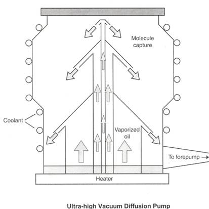
Vacuum Diffusion Pump

Vacuum is created in a chamber using a Vacuum Diffusion Pump (Vapor Jet Pump) like the one pictured:

Picture borrowed from Inside a Vacuum Diffusion Pump

Such a pump can create a vacuum down to 10-10 torr in pressure. However, before this pump can begin its work, another pump, called the roughing or forepump is used to reduce pressure down to 10-3 torr in the glass chamber. At this point the vaccum diffusion pump is started and the pressure starts to drop below 10-3 torr. The reason for this is that the diffusion pump cannot exhaust directly to atmospheric pressure and so the forepump is used to maintain proper discharge pressure conditions.

The way this pump works is that there are three jet assemblies of diminishing sizes as shown in the picture with oil at the base. A heater vaporizes the oil that exits from these jet assemblies and is suddenly cooled by the surrounding coolant, specifically liquid nitrogen in our case which is poured into the system when creating a vacuum. Liquid nitrogen has a temperature of -196 degrees Celsius. “The droplets of oil coming down may actually exceed the speed of sound, but there is no sonic boom, largely because the molecules in partial vacuum are too far apart to transmit the sound energy.” (Joaquim 3) This very high velocity jet stream conveys a downward motion on the molecules bringing them towards the forepump outlet where the gases are removed by the forepump and the condensed oil begins another cycle. Advantages of using this pump are that it is one of the most reliable ways of creating a 10-3 to 10-8 torr vacuum, it lasts for more than thirty years and it has no mechanical parts.

Introduction to the Basic Lock-In

A lock in amplifier is used to detect and measure extremely small AC signals (down to a few nano volts. They allow us to make accurate measurement of small signals even in the presence of thousands of times larger noise signals by using a phase sensitive detection technique that signals out a signal of a specific reference frequency and phase.

We can use this technique because typical experiments are excited at fixed frequency from an oscillator or function-generator.

There is a tutorial about the basic operation of the Lock-In in the Lock-In Manual.

Why Use a Lock-In

In the notebook, I’ve shown calculations of why at 1.6mV of noise we cannot measure 10uV of an output signal by simply using a very good low noise amplifier (100 kHz at 1000 Gain). Then, I’ve shown that not even using a low noise differential amplifier followed by a very good band pass filter centered at 10 kHz still doesn’t work. With this system we get 50uV noise on a 10uV signal.

This is why we need to use a lock-in which is an amplifier with a phase sensitive detector (PSD) which can detect the signal at 10 kHz with a bandwidth as narrow as 0.01 Hz, so that the noise will only be 0.5uV. Now, the signal at 10uV can be accurately measured.

Phase Sensitive Detection (PSD)

Say, reference signal is a square wave at frequency w_r coming from an oscillator or function generator used to excite an experiment that results in a sine wave signal V_sigsin(w_rt + θ_sig)

Another, sine wave V_Lsin(w_Lt + θ_ref) is generated internally by the SR830 (our Lock-In).

The SR830 amplifies the signal and multiplies it with Lock-in reference using PSD or multiplier.

V_psd = V_sigV_Lsin(w_rt + θ_sig)sin(w_Lt + θ_ref) = ½ V_sigV_Lcos([w_r – w_L]t + θ_sig – θ_ref) – ½ V_sigV_Lcos([w_r + w_L]t + θ_sig – θ_ref)

The PSD output is AC signals at the sum and difference frequencies, and when the w_r = w_L we can distinguish it by using a low pass filter on the PSD output resulting in a filtered output.

V_psd = ½ V_sigV_Lcos(θ_sig – θ_ref)

This is a very nice DC signal proportional to the signal amplitude.

Experimental Setup and Procedure

The main parts of this experiment are the thin film deposition in which we deposited 300Angstrom and 600Angstrom Aluminum films onto glass slides. The films were masked to create 3 strips of aluminum on the glass. The mask is shown in a figure in the Shadow Mask section of the lab report.

The second part of this experiment was the four wire measurement. Using the four wire measurement, we measured the current flow across the thin aluminum film strips, in order to determine the resistivity of the aluminum.

Also, before we began we did a small experiment of using the lock-in to determine the resistance of a known resistor. This helped us learn the operation of the lock-in, so that we could then go ahead and use it to measure our thin aluminum films.

Thin Film Deposition

We have already discussed what thin film deposition is and the methods by which it can be achieved. In our case we use thermal evaporation and that too has been discussed. So here is the procedure:

We begin by cleaning the mask and venting the vacuum chamber. We then take off the implosion cover and bell jar, clean the bell jar rim and apply vacuum grease to it. We then load the glass slide and mask into the chamber, and load the boat with aluminum and set it into the chamber and screw it in. We close the vent.

Then we turned on the water, which we could have also turned on earlier, so that we could have started the diffusion pump earlier. We turn on the diffusion pump; close the bell jar and implosion cover. We closed the roughing pump, and opened the backing valve and waited 15 minutes for the diffusion pump. We then closed the backing, opened the roughing and waited 5-6 minutes. Then we powered on the cold cathode gauge, closed the roughing and open backing pump. We open the closet lever and kept the vacuum gauge on high voltage (base pressure 1.9x10-4 torr). On the deposition controller (INFICON XTC/2) we set the thickness of the evaporation source. Finally, we turn on the power supply and let the deposition occur.

Our base pressure was 2.8x10^-5 torr. We deposited 600Angstrom and 300Angstrom aluminum films with this procedure.

Finally, we close the gate valve, close diffusion pump, and turn rotary pump on, switch off high voltage gauge. Then, we turn off power supply breaker, and let the water still run. We open the vent and take out our sample.

Four Wire Measurement

We start by attaching wires using Indium to our aluminum on the glass slide shown with the masked aluminum thin films so that we can measure the resistance of the 3 aluminum strips on the 600Angstrom and the 300Angstrom films. I call the widest strip 0.09in AL1, the medium strip AL2 (0.06in), and the thinnest strip AL3 (0.03in). We measure the resistance using the lock-in amplifier as previously described to measure the I-V curves. The procedure to attach the Indium is to cut a small piece of it using a razor from the Indium roll and slice it in two halves. Then use a cotton swab to press one of the halves into position in the Aluminum.

Next, put a wire on it and sandwich it between the indium using the other half so it sticks in. Making good contacts but no shorts is important.

Four Wire measurements:

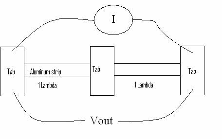
Shown is the setup for the four wire measurement for two lambdas. There are tabs in our strips. From one tab to the next is one lambda. The lock-in provides the output voltage sine wave, which is passed across a 1MOhm resistor to produce a current, I. Vout is then measured by the lock-in and the calculations previously discussed are performed by the lock-in.

Shadow Mask

See the attached blueprint of the Shadow mask. It shows the exact dimensions, locations of tabs etc.

Data and Calculation of Resistivity

Length and Width vs. Resistance Plots

Data and Calculations

Vin (V)	Vout (uV)	Vout (v)		I (A)	Vout	Rx
1	0.04488	0.00004488	0.000001	9.6242E-07	4.52338E-05	46.632429
1.5	0.06729	0.00006729	0.0000015	1.44363E-06	6.78506E-05	46.611648	1039000
2	0.08962	0.00008962	0.000002	1.92484E-06	9.04675E-05	46.559696	47
2.5	0.11209	0.00011209	0.0000025	2.40605E-06	0.000113084	46.586711	1039047
3	0.13456	0.00013456	0.000003	2.88726E-06	0.000135701	46.604721
3.5	0.15797	0.00015797	0.0000035	3.36847E-06	0.000158318	46.896644
4	0.17947	0.00017947	0.000004	3.84968E-06	0.000180935	46.619441
4.5	0.2019	0.0002019	0.0000045	4.33089E-06	0.000203552	46.618575
5	0.2243	0.0002243	0.000005	4.8121E-06	0.000226169	46.611648

Area(1)	Area (2)	Area (3)
2.29E-11	2.286E-11	2.286E-11
4.57E-11	4.572E-11	4.572E-11
6.86E-11	6.858E-11	6.858E-11
Area/ thickness	A/T	A/T
2.25E-09	1.125E-09	7.5E-10
4.5E-09	2.25E-09	1.5E-09
6.75E-09	3.375E-09	2.25E-09
	L (cm)	L (m)		Area(1)	Area (2)	Area (3)
0.03	0.0762	0.000762		4.572E-11	4.572E-11	4.572E-11
0.06	0.1524	0.001524		9.144E-11	9.144E-11	9.144E-11
0.09	0.2286	0.002286		1.3716E-10	1.3716E-10	1.372E-10
				Area/thickness	A/T	A/T
0.03				4.5E-09	2.25E-09	1.5E-09
0.06				0.000000009	4.5E-09	3E-09
0.09				1.35E-08	6.75E-09	4.5E-09


600A
0.09							4.572E-11
600 A	Vin	Vo(uV)	Vo (v)	I	Rx	p	9.144E-11
3	1	10.3	0.0000103	9.62464E-07	10.7017	4.816E-08	1.3716E-10
lambda	2	20.6	0.0000206	1.92493E-06	10.7017	4.816E-08
300A				0
				0			2.286E-11
2	1	6.6	0.0000066	9.62464E-07	6.8574	4.629E-08	4.572E-11
	2	13.35	0.00001335	1.92493E-06	6.935325	4.681E-08	6.858E-11
1	1	3.5	0.0000035	9.62464E-07	3.6365	4.909E-08
	2	6.9	0.0000069	1.92493E-06	3.58455	4.839E-08
0.06				0
1	1	4.2	0.0000042	9.62464E-07	4.3638	3.927E-08
	2	8.5	0.0000085	1.92493E-06	4.41575	3.974E-08
2	1	9.29	0.00000929	9.62464E-07	9.65231	4.344E-08
	2	18.24	0.00001824	1.92493E-06	9.47568	4.264E-08
3	1	13.6	0.0000136	9.62464E-07	14.1304	4.239E-08
	2	27.2	0.0000272	1.92493E-06	14.1304	4.239E-08
0.03				0
1	1	8.59	0.00000859	9.62464E-07	8.92501	4.016E-08
	2	17.14	0.00001714	1.92493E-06	8.90423	4.007E-08
2	1	18.28	0.00001828	9.62464E-07	18.99292	4.273E-08
	2	35.98	0.00003598	1.92493E-06	18.69161	4.206E-08
3	1	36.29	0.00003629	9.62464E-07	37.70531	5.656E-08
	2	73.48	0.00007348	1.92493E-06	38.17286	5.726E-08
300A (0.03 in)				0
1	1	19	0.000019	9.62464E-07	19.741	4.442E-08
	2	38	0.000038	1.92493E-06	19.741	4.442E-08
2	1	35	0.000035	9.62464E-07	36.365	4.091E-08
	2	58	0.000058	1.92493E-06	30.131	3.39E-08
3	1	20	0.00002	9.62464E-07	20.78	4.676E-08
	2	43	0.000043	1.92493E-06	22.3385	5.026E-08
0.06 in				0
1	1	12	0.000012	9.62464E-07	12.468	5.611E-08
	2	26	0.000026	1.92493E-06	13.507	6.078E-08
2	1	20	0.00002	9.62464E-07	20.78	4.676E-08
	2	43	0.000043	1.92493E-06	22.3385	5.026E-08
3	1	38	0.000038	9.62464E-07	39.482	5.922E-08
	2	60	0.00006	1.92493E-06	31.17	4.676E-08
0.09 in				0
1	1	7.06	0.00000706	9.62464E-07	7.33534	4.951E-08
	2	14.37	0.00001437	1.92493E-06	7.465215	5.039E-08
2	1	14.3	0.0000143	9.62464E-07	14.8577	5.014E-08
	2	29.11	0.00002911	1.92493E-06	15.122645	5.104E-08
3	1	22.33	0.00002233	9.62464E-07	23.20087	5.22E-08
	2	44.2	0.0000442	1.92493E-06	22.9619	5.166E-08

600Ang.									Rho	Fract-ional Error
0.09	# of strips	strip L	strip A	Strip (L/A)	# of tabs	Tab (L/A)	total L/A	R	R*A/L
3	3	0.009093	1.3716E-10	66296296	2	5.58E+06	2.10E+08	10.7017	5.09E-08	-0.02841
2	2	0.009373	1.3716E-10	68333333	1	5.58E+06	1.42E+08	6.8574	4.82E-08	-0.01989
1	1	0.01016	1.3716E-10	74074074	0	5.58E+06	7.41E+07	3.6365	4.91E-08	0.001296

0.06	# of strips			Strip (L/A)	# of tabs	Tab (L/A)	total L/A	R	R*A/L
3	3	0.009093	9.144E-11	99444444	2	5.58E+06	3.09E+08	14.1304	4.57E-08	-0.03067
2	2	0.009373	9.144E-11	1.03E+08	1	5.58E+06	2.11E+08	9.65231	4.58E-08	-0.02411
1	1	0.01016	9.144E-11	1.11E+08	0	5.58E+06	1.11E+08	4.3638	3.93E-08	-0.00329

0.03	# of strips			Strip (L/A)	# of tabs	Tab (L/A)	total L/A	R	R*A/L
3	3	0.009093	4.572E-11	1.99E+08	2	5.58E+06	6.08E+08	37.70531	6.20E-08	-0.0351
2	2	0.009373	4.572E-11	2.05E+08	1	5.58E+06	4.16E+08	18.99292	4.57E-08	-0.02921
1	1	0.01016	4.572E-11	2.22E+08	0	5.58E+06	2.22E+08	8.92501	4.02E-08	-0.015

300Ang.
0.09	# of strips			Strip (L/A)	# of tabs	Tab (L/A)	total L/A	R	R*A/L
3	3	0.009093	6.858E-11	1.33E+08	2	8.95E-08	3.98E+08	23.20087	5.83E-08	-0.01677
2	2	0.009373	6.858E-11	1.37E+08	1	8.95E-08	2.73E+08	14.8577	5.44E-08	-0.01107
1	1	0.01016	6.858E-11	1.48E+08	0	8.95E-08	1.48E+08	7.33534	4.95E-08	0.004096

0.06	# of strips			Strip (L/A)	# of tabs	Tab (L/A)	total L/A	R	R*A/L
3	3	0.009093	4.572E-11	1.99E+08	2	8.95E-08	5.97E+08	39.482	6.62E-08	-0.01855
2	2	0.009373	4.572E-11	2.05E+08	1	8.95E-08	4.10E+08	20.78	5.07E-08	-0.01299
1	1	0.01016	4.572E-11	2.22E+08	0	8.95E-08	2.22E+08	12.468	5.61E-08	-0.00152

0.03	# of strips			Strip (L/A)	# of tabs	Tab (L/A)	total L/A	R	R*A/L
3	3	0.009093	2.286E-11	3.98E+08	2	8.95E-08	1.19E+09	44.677	3.74E-08	-0.01885
2	2	0.009373	2.286E-11	4.1E+08	1	8.95E-08	8.20E+08	36.365	4.43E-08	-0.01506
1	1	0.01016	2.286E-11	4.44E+08	0	8.95E-08	4.44E+08	19.741	4.44E-08	-0.00447

Resistivity without Accounting for Tabs

Resistivities
lambda	600A 1 strip	600A 2 strip	600A 3 strip	300A 1 strip	300A 2 strip	300A 3 strip
1	4.91E-08	3.93E-08	4.02E-08	4.95E-08	5.61E-08	4.44E-08
2	4.63E-08	4.34E-08	4.27E-08	5.01E-08	4.68E-08	4.09E-08
3	4.82E-08	4.24E-08	5.66E-08	5.22E-08	5.92E-08	4.68E-08

Resistivity Accounting for the Tabs

Resistivities accounting for tabs
lambda	600A 1 strip	600A 2 strip	600A 3 strip	300A 1 strip	300A 2 strip	300A 3 strip
1	4.91E-08	3.93E-08	4.02E-08	4.95E-08	5.61E-08	4.44E-08
2	4.82E-08	4.58E-08	4.57E-08	5.44E-08	5.07E-08	4.43E-08
3	5.09E-08	4.57E-08	6.20E-08	4.95E-08	6.62E-08	3.74E-08

Model as Resistance in Series

We model the aluminum strips and the tabs within them as resistances in series. The resistivity is then calculated using the formula R = Rho*L/A where R is the resistance, Rho is the resistivity, length is the length the current travels and A is the cross sectional area of the strip or the tab. We know all the physical dimensions of the strip or tab and we also know the measured resistances, so we are able to determine resistivities as seen in the data tables.

Error Analysis

Impurities

The theoretical value for the resistivity of pure aluminum is 2.8x10^-8 ohm meters. In our thin film aluminum there are impurities so our resistivity is higher than the theoretical resistivity determined for a pure aluminum crystal. In fact, it is almost double, on the order of 4 to 6x10^-8 ohm meters as seen by the values in the data table.

Fractional Error

The fractional errors are calculated for each of the resistivities calculated when accounting for the tabs. They are in the table. We can see the fractional uncertainty for the 600Angstrom film is about -2% on average and for the 300Angstrom film is about -1%. This difference is because I estimated an error of about 10Angstroms in the deposition process, and so for a film half as thick, the error would be twice as much. Since in calculating the resistivity, this thickness is multiplied by as part of the cross sectional area, this error is added in with other fractional uncertainties in the resistivity calculation. The fractional errors are negative, so the fractional uncertainty in the 300Angstrom film caused the number to become smaller. They are negative because the biggest source of fractional uncertainty is the length measurement of the strip. The length measurement is divided by in the formula ρ = R*A/L.

Error sources include the measurement of the thickness of the thin film as there might be some extra film deposited or not enough film deposited in terms of when the heater was stopped and started. There might be error due to fluctuation in reading the lock-in although it is a pretty good device. The numbers on the mask blueprint might not be exact in terms of calculating the strip dimensions.

Conclusions

From the resistance vs. length graphs we can see that the resistance increases with increasing length, which is clearly what it should do as R = ρL/A.

On the other hand from the resistance versus width graphs we can see the inverse relation as for a thin film of constant thickness the Area, A is directly proportional to the width and again R = ρL/A.

We analyzed that the calculated values of the resistivities are almost double, than the theoretical values due to impurities in the aluminum, from that of a single ideal aluminum crystal.

Tab Accounting

Comparing the values with accounting for the tabs with the ones without accounting for the tabs we don’t see much discrepancy although comparing individual values we note that accounting for the tabs increased our calculated resistivities. This is because the tabs have a lower resistance than the strips. Since, the resistance is lower; there would be more current flow for the given voltage given a substance of some resistivity. Since, we are calculating the resistivity and the current is still measured to be what we measured it to be, our calculated resistivity goes up, when we account for the tabs.

From my graphs, however, I am not seeing the dependence of length on the resistivity when we don’t account for the tabs, due to the tabs.

300Angstrom versus 600Angstrom

When we compare the resistivities calculated from the 300Angstrom against those calculated with the 600Angstrom, we notice that there is more spread in the measurement from the 300Angstrom. That is ignoring accuracy; the 600Angstrom data is more precise. Possibly, this is because the surface impurities in the 300Angstrom make more of an effect, whereas the impurities within the 600Angstrom are more evenly dispersed.

Also, according to Fuchs model, the measured resistivity of bulk aluminum should decrease and get closer to the theoretical value of 2.7 as the thickness is increased. Accordingly, the 600Angstrom should be closer to the theoretical value.

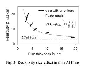Image from: http://www.rpi.edu/~schowl/mbe-research/al-size.html