Aditya Mittal March 02, 2007
NMR Lab Experimental Physics II
Introduction
We began this experiment by familiarizing ourselves with the NMR equipment, Teach Spin’s PS1-A which is the first pulsed nuclear magnetic resonance spectrometer designed for teaching. The pulse nuclear magnetic resonance begins with a net magnetization of the protons aligned in the +z direction of a sample in thermal equilibrium in a strong magnetic field from a permanent magnet. The alignment is altered by one or more 90 or 180 degree radio frequency pulses, by tipping the spins in the x-y plane and letting it precess around the z direction creating a time varying voltage in a pick up coil, which monitors the magnetization in the x-y plane.
The receiver amplifies the signal coming from the pickup coil which is an induced voltage sine wave rising and falling with each rotation. Some damping of the sine wave occurs due to the interactions between the lattice and the spin as well as due to the interactions between the spin and the spin. Eventually the signals decay to zero voltage, as the precession stops and the protons are again aligned in the +z direction.
The signal from the receiver is rectified so that only a positive magnitude is shown each time and it is this rectified envelope which represents the free induction decay or FID. We measure this FID on the oscilloscope through the detector out port. Through measuring the signals we are then able to proceed to determine the spin-lattice relaxation time and the spin-spin relaxation time of a given sample such as mineral oil or glycerin. Relaxation time as the name implies is the time it takes these sine waves to decay.
Other important parameters that can be set with the instrumentation include the number of pulses, delay time, repetition time, pulse width, and gain.
Apparatus
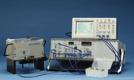
The above picture shows the apparatus. The box to the left is the magnet. It is connected by the blue BNC cables, to another box which has three sections. The first of these three sections is the receiver, the second is the pulse programmer, and the third is the oscillator and mixer. On top of this box is the oscilloscope. Below in the little semitransparent box are little tubes of test samples. In our case we use mineral oil and glycerin.
Procedure (See lab
sheet for details – this is just an outline)
- Learning the Apparatus – in this part
we explore the instrument, setup and calibrate the equipment
- Pulse Programmer
i.
Single Pulse
ii.
The Pulse
Sequence
iii.
Multiple
Pulse Sequence
- Receiver
- Spectrometer
- Single Pulse NMR Experiment – free
precession induction decay
- Magnetic field contours
- Determining T1, the
spin-lattice relaxation time
- The spin-lattice relaxation time is
the time constant that characterizes the exponential growth of the
magnetization towards thermal equilibrium in a static magnetic field. We began by doing a quick estimate of T1
by setting the FID pulse to its maximum amplitude and then reducing it to
a third of the value by reducing the repetition time. This repetition time is representative
of T1.
- Next we went ahead and measured T1
using the Two Pulse – Zero Crossing method in which we set up a two pulse
sequence that went 180 degree A pulse, then wait for time tau, and then a 90 degree B pulse and again wait for
time tau.
- Determining T2, the
spin-spin relaxation time
- Two pulse spin echo
- Multiple pulse multiple spin echo
sequences
i.
Carr-Purcell
ii.
Meiboom-Gill
We repeated the experiment procedures with mineral oil and glycerin.
Learning the Apparatus
Pulse Programmer
We began by investigating the pulse programmer. We generated different pulses with different amplitudes and delay times. The pulse programmer is the middle unit in the three units on the NMR apparatus. We generated single pulse by creating an A pulse. Then we went ahead and created a pulse sequence with both A and B pulse, and finally we made multiple pulse sequences by turning on A pulse and then setting the number of B pulses to more than 1. We made sequences such as 5 pulse sequences by making 1 A pulse and 4 B pulses.
Receiver
The receiver took its inputs from the pickup coil in the permanent magnet and outputted to the mixer and the RF Amplifier Detector circuit. The mixer signal and the RF Amplifier Detector circuits were both seen on the oscilloscope. The frequency of the oscillator on the 3rd unit in the apparatus was adjusted so that the mixer signal had no beats in order to set the frequency to the magnet’s resonant frequency. In this initial experiment we used the dummy signal probe to tune the receiver and observe the rf and detected signals as a function of tuning and gain.
Spectrometer
In this section we connected the BNC cables and setup all the instrumentation to prepare for the actual measurements with glycerin and mineral oil. We also connected the blanking pulse incase our samples had a very short T2.
Single Pulse NMR
Experiment – free precession induction decay
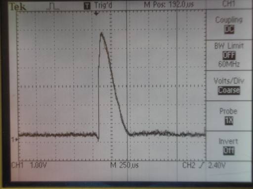
We look for our first FID signal with a single RF pulse in this part. We began by waiting for the thermal equilibrium to get established with our mineral oil sample inside the magnet. We set up the parameters mentioned in the lab procedure for the pulse programmer so we could view the FID of mineral oil. We found the 90 degree pulse A-width by looking for where the FID signal from the rf amplifier detector was highest. The FID signal from the amplifier detector of the mineral oil is shown in this photograph.
Magnetic field contours
In this part of the lab we went ahead and found the resonance frequencies in all the different parts of the magnet with the mineral oil by eliminating the beats against the master oscillator’s frequency using the mixer. We plotted the frequency versus the x position as well as against the y position to map out our permanent magnet. The two graphs and their data are shown:
By Rot the Y position is meant, as it was changed by rotating the knob on the magnet. The Y values were taken for x = 0.
|
x=0 |
|
|
|
|
|
|
|
|
Rot |
f
(MHz) |
|
|
|
X |
f
(MHz) |
|
|
0 |
15.33252 |
15.3288 |
|
|
-3 |
15.61924 |
15.3288 |
|
1 |
15.32885 |
15.3288 |
|
|
-2 |
15.52106 |
15.3288 |
|
2 |
15.3327 |
15.3288 |
|
|
-1 |
15.42351 |
15.3288 |
|
3 |
15.34287 |
15.3288 |
|
|
0 |
15.32885 |
15.3288 |
|
4 |
15.35273 |
15.3288 |
|
|
1 |
15.34894 |
15.3288 |
|
5 |
15.36259 |
15.3288 |
|
|
2 |
15.39708 |
15.3288 |
|
6 |
15.36343 |
15.3288 |
|
|
3 |
15.48554 |
15.3288 |
|
|
|
|
|
|
|
|
|
|
|
fo - 4.258(3.6)= 15.3288 (MHz) |
|
|
|
|
||
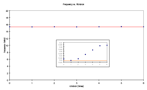
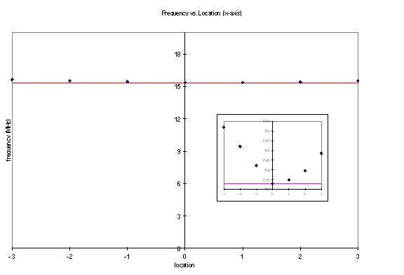
The two graphs show our mapping of the magnet as talked about. The “sweet spot” in our magnet lies at x = 0.0 and Rot = 1.1 and it’s where we get the best FID graph.
Determining T1, the spin-lattice relaxation
time
The spin-lattice
relaxation time is the time constant that characterizes the exponential growth
of the magnetization towards thermal equilibrium in a static magnetic
field. We began by doing a quick
estimate of T1 by setting the FID pulse to its maximum amplitude and
then reducing it to a third of the value by reducing the repetition time. This repetition time is representative of the
order of magnitude of T1.
For the mineral oil we got this value to be 4ms as reducing the repetition time from 80ms to 4ms made the largest value of 5.80V go to 1/3(5.80V) = 1.93V. This allowed us to know that we were looking for a mineral oil spin-lattice relaxation time on the order of a few milliseconds.
Next we went ahead
and measured T1 using the Two Pulse – Zero Crossing method in which
we set up a two pulse sequence that went 180 degree A pulse, then wait for time
τ, and then a 90 degree B pulse and again wait for the delay time, τ.
Using the Origin program we plotted our data, and Origin gave us a value for T1 of Mineral Oil as 13 ms, which is close enough to the listed value of 12ms in our lab packet. I am unable to attach the graphs with the report at this moment because I do not have the origin software here.
In a similar manner, we measured the T1 of Glycerin and got a value of T1 from Origin to be 50ms. We do not know or have an estimate of the actual or expected value.
Determining T2, the spin-spin relaxation
time
T1
was the spin-lattice relaxation time, which was the decay of the longitudinal
magnetization of the system. T2
on the other hand is the spin-spin relaxation time and is the transverse magnetization
of the system. In order to measure T2
we must use a 90 degree pulse to create a longitudinal magnetization as
transverse magnetization cannot directly be measured. Therefore, whenever we want to measure the
transverse magnetization, we will turn it 90 degrees and measure the resulting
pulse immediately after.
A spin echo experiment is needed if
T2 is greater than 0.3 ms to get an accurate value of T2
due to imperfections in even the really good magnet. For values smaller, the FID decay time constant
gives a good estimate.
Two pulse spin echo
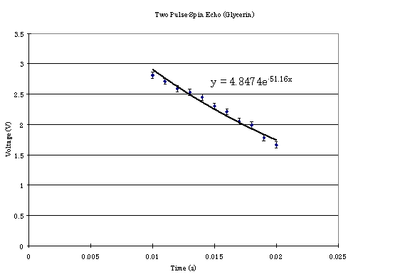
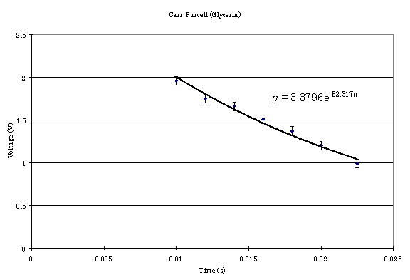
In the two pulse spin echo we setup a 90 degree pulse followed by a 180 degree pulse after some time constant, and we wait for two time constants after the 180 degree pulse. This causes the reversal of the x-y magnetization and a rephrasing of the spins at a later time. This method was discovered by Irwin Hahn in 1950 in order to compensate for the apparent decay in the x-y magnetization due to inhomogeneity of an external magnetic field as discussed above. There are two ways to explore the magnitude of T2. One is to vary the delay time between the A and the B pulse by plotting the resulting echo maximum as a function of time. The other is to introduce a series of 180 degree B pulses and look at the decrease of the maxima, as we shall do in the next part.
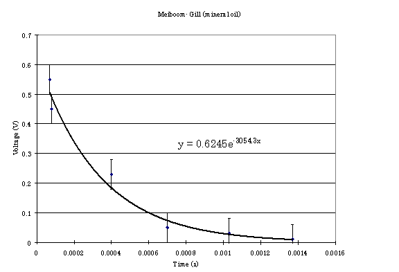
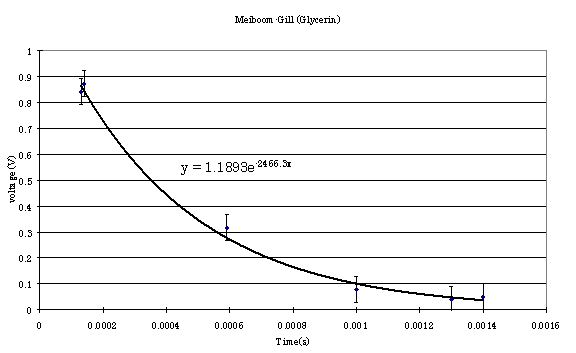
Shown below are our graphs for the mineral oil and glycerin for the two pulse spin echo. T2 is inversely proportional to the exponent in the equations as the magnetization equation reads like Mx or y(t) = M0e-t/T2.
Multiple-pulse
multiple spin echo sequences
As discussed already, the second method of using spin echo to determine T2 is to introduce a series of 180 degree B pulses and look at the decrease of the maxima. There are two possibilities within this method. Carr-Purcell and then Meiboom Gill which performs an additional correction for the error caused due to the practical inability to get an exact 180 degree pulse.
The advantage of the multiple spin-echo sequence method over the single spin-echo sequence method is that the multiple spin-echo sequence reduces the effect of self diffusion, an experiment we did not do due to lack of time.
Carr-Purcell
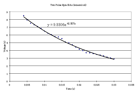
This is the standard multiple spin-echo sequence method we talked about. It was devised by Carr and Purcell. In this method multiple 180 degree pulse sequence is applied spaced by a delay time. So as the NMR equipment does it applies the A-pulse, then some delay, then series of B pulses with twice the delay between the A and first B pulse we produce a 90 degree A pulse followed by half time constant followed by 180 degree B pulses with one time constant between each. The echo envelope’s maximum height is then used to calculate T2. As we are trying to reduce the self-diffusion error the time constant should be small compared to the self-diffusion time of the spins through the field gradients. Following are the two graphs we got from the Carr-Purcell method for Mineral Oil and Glycerin:
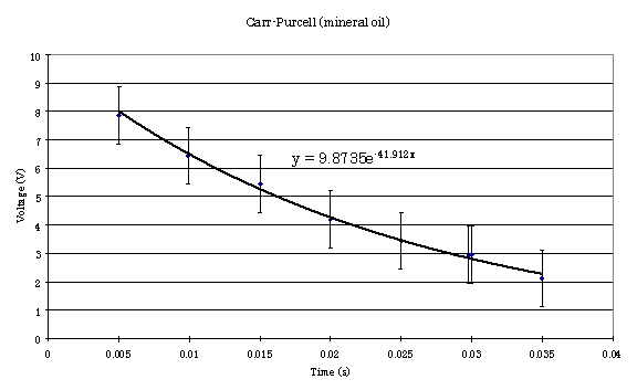
The values of the two pulse and multiple pulse sequences in our case are almost the same. This means that either the self diffusion was not corrected due to a large delay time compared to the self diffusion constant or the two pulse sequence gave us good enough results as well. We don’t know the value for self diffusion for our samples, so we cannot say.
Meiboom-Gill
Finally, we did the Meiboom-Gill method of measuring T2 to eliminate the serious practical problem of 180 degree pulses not really being 180 degrees. In this experiment we consider the fact that if the spectrometer is producing say 183 degree pulses, by the time the 20th pulse is turned on the spectrometer would have accumulated a rotational error of 60 degrees giving seriously erred value of T2. This is exactly what happened. From the method of Meiboom-Gill we were able to get a corrected value on our graphs, which is totally different from the values calculated by the two-pulse and Carr-Purcell methods. The trick to Meiboom and Gilll’s method is that between every 90 degrees and 180 degrees pulses they phase shift the system by 90 degrees canceling the error to first order. Therefore, all real data for T2 should be calculated with the M-G pulse on. So here are our graphs from the Meiboom-Gill experiment for both mineral oil and glycerin. Notice, the equations are very different from before, and more accurate too.
Conclusions
In this experiment we learnt how to determine the spin-lattice and spin-spin relaxation times using the NMR techniques. We got a value close to the expected value of 12ms for the T1 of mineral oil. We do not know the T2 values for Glycerin or Mineral Oil, and we also do not know the T1 value for Glycerin. So, we could not compare to other people’s values. We had fun.